Volume Decomposition Using Panel Data: Why Are Sales Up or Down?

Many people are familiar with the analysis known as a volume decomposition (or due-to) that uses POS data.  This allows you to explain a change in sales and attribute gains and losses to specific business drivers like distribution, pricing, trade promotion and some other things.  We have a series of posts on this, starting with this one that also has links to the other posts in the series.

There is another way to explain a change in sales using household panel data.  (Take a look at this post if you need a refresher on panel data.)

The usual reason for doing a sales decomp is to explain why sales are down, but this can also be done to explain why sales are up.  Panel data lets you quantify how much of a sales decline is because of fewer householder buying the product (penetration) vs. the same number of households buying less (buy rate).  As a next step, if shoppers are buying less, you can determine how much change is because of purchase frequency vs. purchase size.  This post addresses the high level decomp of penetration vs. buy rate.  I’ll focus on volume buy rate in this example.  (See this post about the 3 ways to measure sales – dollars, units and equivalized volume or EQ.)

The analysis starts by looking at change in sales from one period to another.  As with most panel data analyses, you typically look at one year vs. the previous year.  Shorter periods can be a problem if the penetration or purchase cycle for the product is low, i.e. people only buy it a few times a year.  This is especially true for household and personal care products.  It is virtually impossible to have a large enough sample size in panel data to look at any individual SKU.  (Note that this is not an issue when doing a decomp using POS data, as sales data is always available at all product levels in that data source.)

Cereal Brand Example

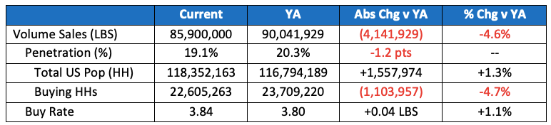
We’ll use the following real data for this example (although from 10+ years ago).  It’s for a nationally distributed ready-to-eat cereal brand from a major manufacturer.

This is what we’re looking at:

• Product is the total brand Fun Flakes
• Market is Total US All Outlet (as defined back in 2012)
• Period is one full year ending early November 2012
• Volume is measured in pounds (LBS), the EQ (equivalized unit) that takes into account different package sizes offered by the brand
• Note that calculations were done prior to rounding

Here’s a quick overview of what’s happening here:

1. Volume is down -4.6%, just over 4 million pounds from a year ago.
2. Just over 19% of all US households bought Fun Flakes at least one time during the year but that’s down over 1 point. (Note that we do not show the % change in penetration since that measure is already a percentage.)
3. Buy rate is up slightly (+1.1%), with the average household (HH) buying just under 4 LBS in a year.
4. A gain in purchase frequency is slightly offsetting a decline in purchase size.
5. The average annual buy rate of 3.8 LBS breaks into the average HH buying Fun Flakes 3 times per year (up from last year), 1.3 LBS per trip (down from last year).

Objective of Due-To Analysis

This analysis allows you to allocate the 4.1 million pound volume decline between buyers and buy rate.  Depending on the responsible driver(s) you would use different marketing tactics to hopefully fix the issue.

* A brand can increase its penetration and/or buy rate by expanding into other channels. Say, for example, that Brand X gains distribution in the Club channel for the first time.  Penetration could increase among shoppers who only buy the category in Club and now see Brand X there.  Buy rate could also increase since shoppers who already buy the brand in other channels can now buy it on more of their shopping trips (at Club)

You need to consider trade-off of cost vs. benefit – is it easier/cheaper to get a new or lapsed buyer or to increase purchases among existing buyers?

Due-To Calculations

In order to allocate a volume change between buyers and buy rate, the key thing is to allow one element to change while the other stays the same.

Slight but necessary detour:
When doing these calculations, it’s not enough to just look at penetration.  You also need the actual number of households who purchased to accurately estimate volume.  This is because the number of total households in the US changes from year to year, in addition to the Penetration changing.  In this example 19.1% penetration translates into 22.6 million households who bought Fun Flakes:  There were 118.4 million total households in the US back in 2012 (current year in the example) so 0.191 * 118,400,000 = 22.6 million households.  In the year ago period 2011, penetration of 20.3% and 116.8 million total US households means there were 23.7 million households (0.203 * 116,800,000) who bought the brand in the previous year.  So…buying households decreased by -1.1 million or -4.7%.

Here is the data used in the analysis:

The key concept is that you assume one change but everything else stayed the same.

LBS due-to

• LBS change due-to Buyers
  Change in Buyers * Current Buy Rate
  (Current Buyers – YA Buyers) * Current Buy Rate
  (22.6MM – 23.7MM) * 3.84 LBS = -4.2 MM LBS
• LBS change due-to Buy Rate
  Change in Buy Rate * Current Buyers
  (Current Buy Rate – YA Buy Rate) * Current Buyers
  (3.84 LBS – 3.80 LBS) * 22.6MM = +900k LBS

% due-to = LBS due-to / YA volume

• % due-to Buyers = -4.2MM / 90.1MM = -4.7%
• % due-to Buy Rate = +900k / 90.1MM = +1.0%

It is not a coincidence that the sum of the % due-to in buyers and buy rate is close to the % change in volume (-4.7% + 1.0% is close to -3.7%)!  Sometimes it’s off slightly due to rounding, plus some small amout due to the change in Total US population.

So to summarize…we see that loss of buyers was responsible for more than the -4.6% volume decline (-4.7%, or -4.2 million LBS) while the slight increase in buy rate actually offset this by +1.1%, or +900k LBS.  Note:  It is very common for buy rate to increase when penetration decreases because the buyers that leave are typically lighter buyers and the ones that stay have a higher buy rate.

Did you find this article useful?  Subscribe to CPG Data Tip Sheet to get future posts delivered to your email in-box. We publish new articles on an ad hoc basis and do respond to comments and questions.